The simplest 2D plot is plot(x,y) or plot(y): this is the plot of y as function of x where x and y are 2 vectors; if x is missing, it is replaced by the vector (1,...,size(y)). If y is a matrix, its rows are plotted. There are optional arguments.
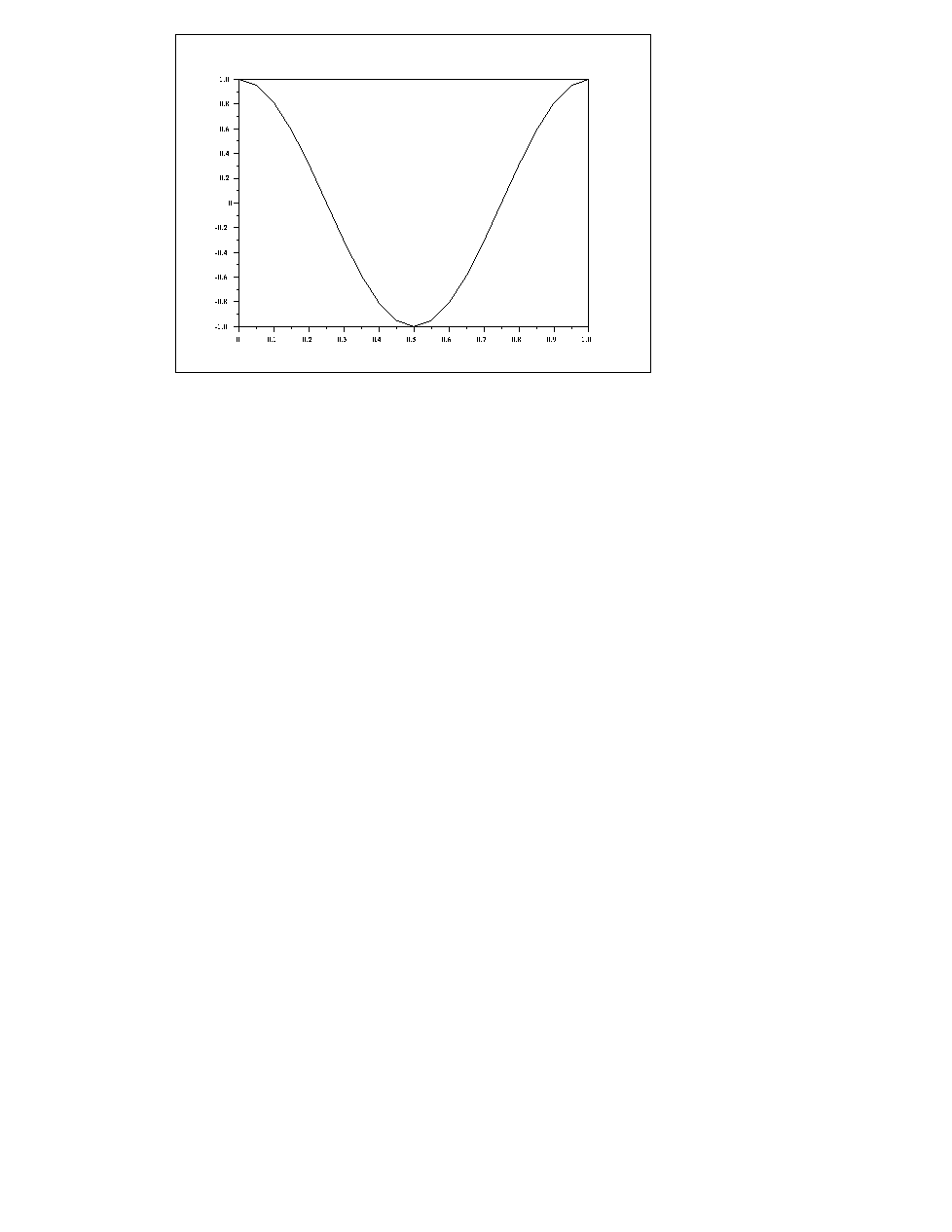
A first example is given by the following commands and one of the results is represented on figure 5.1:
t=(0:0.05:1)';
ct=cos(2*%pi*t);
// plot the cosine
plot(t,ct);
// xset() opens the toggle panel and
// some parameters can be changed with mouse clicks
// given by commands for the demo here
xset("font",5,4);xset("thickness",3);
// plot with captions for the axis and a title for the plot
// if a caption is empty the argument ' ' is needed
plot(t,ct,'Time','Cosine','Simple Plot');
// click on a color of the xset toggle panel and do the previous plot again
// to get the title in the chosen color
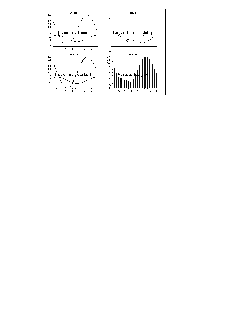
The generic 2D multiple plot is
plot2di(str,x,y,[style,strf,leg,rect,nax])
plot2d : i=missing,1,2,3,4.
For the different values of i we have:
i=missing : piecewise linear plotting
i=1 : as previous with possible logarithmic scales
i=2 : piecewise constant drawing style
i=3 : vertical bars
i=4 : arrows style (e.g. ode in a phase space)
t=(1:0.1:8)';xset("font",2,3);
xsetech([0.,0.,0.5,0.5],[-1,1,-1,1]);
plot2d([t t],[1.5+0.2*sin(t) 2+cos(t)]);
xtitle('Plot2d');
titlepage('Piecewise linear');
//
xsetech([0.5,0.,0.5,0.5],[-1,1,-1,1]);
plot2d1('oll',t,[1.5+0.2*sin(t) 2+cos(t)]);
xtitle('Plot2d1');
titlepage('Logarithmic scale(s)');
//
xsetech([0.,0.5,0.5,0.5],[-1,1,-1,1]);
plot2d2('onn',t,[1.5+0.2*sin(t) 2+cos(t)]);
xtitle('Plot2d2');
titlepage('Piecewise constant');
//
xsetech([0.5,0.5,0.5,0.5],[-1,1,-1,1]);
plot2d3('onn',t,[1.5+0.2*sin(t) 2+cos(t)]);
xtitle('Plot2d3')
titlepage('Vertical bar plot')
xset('default')
Figdirfigures/
a=e : means empty; the values of x are not used; (The user must give a dummy value to x).
a=o : means one; the x-values are the same for all the curves
a=g : means general.
b=l : a logarithmic scale is used on the X-axis
c=l : a logarithmic scale is used on the Y-axis
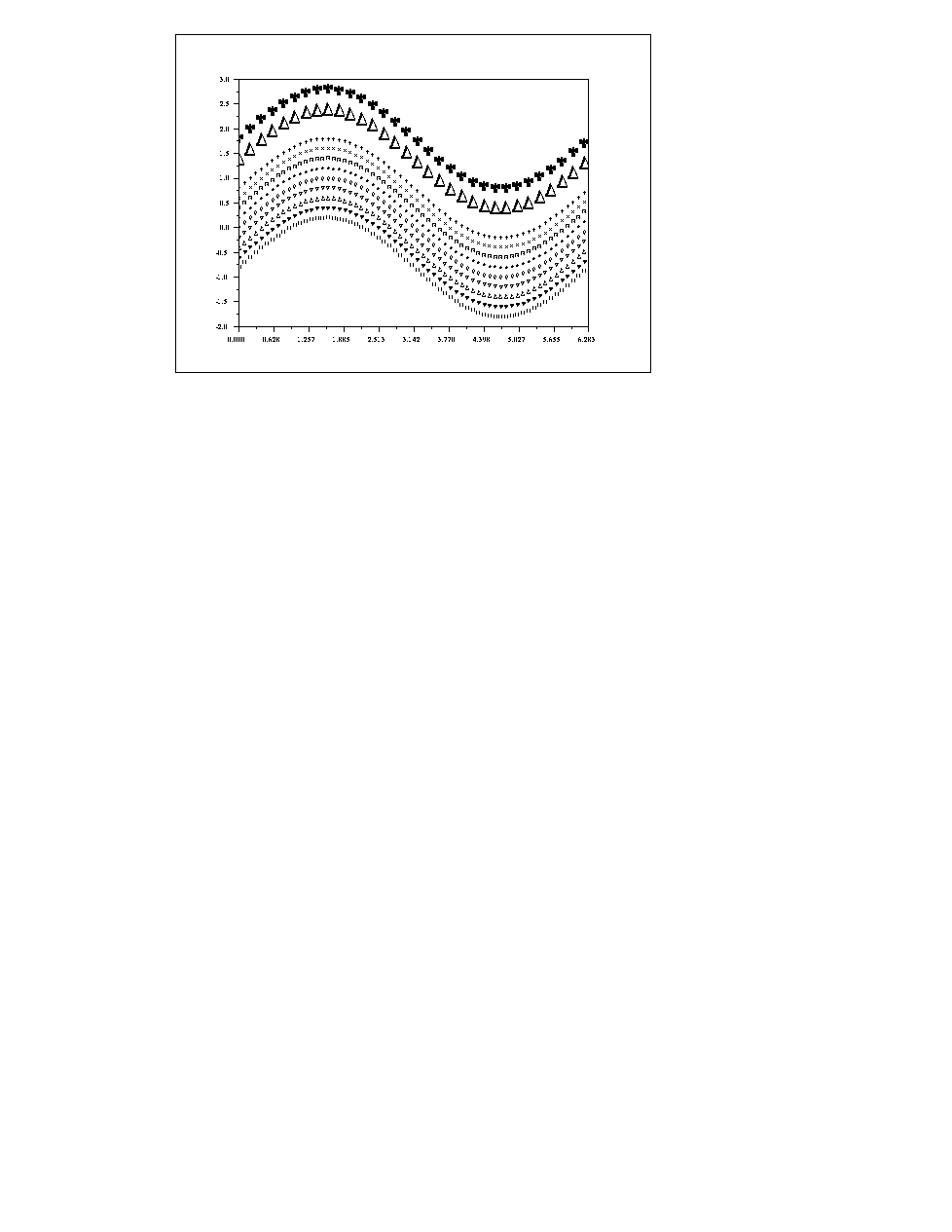
-Parameters x,y : two matrices of the same size [nl,nc] (nc is the number of curves and nl is the number of points of each curve).
For a single curve the vector can be row or column : plot2d(t',cos(t)') plot2d(t,cos(t)) are equivalent.
x=0:0.1:2*%pi;
u=[-0.8+sin(x);-0.6+sin(x);-0.4+sin(x);-0.2+sin(x);sin(x)];
u=[u;0.2+sin(x);0.4+sin(x);0.6+sin(x);0.8+sin(x)]';
//start trying the color with the 2 following lines
//sty=[-9,-8,-7,-6,-5,-4,-3,-2,-1,0];
//plot2d1('onn',x',u,sty,"111"," ",[0,-2,2*%pi,3],[2,10,2,10]);
plot2d1('onn',x',u,...
  [9,8,7,6,5,4,3,2,1,0],"011"," ",[0,-2,2*%pi,3],[2,10,2,10]);
x=0:0.2:2*%pi;
v=[1.4+sin(x);1.8+sin(x)]';
xset("mark",1,5);
plot2d1('onn',x',v,[7,8],"011"," ",[0,-2,2*%pi,3],[2,10,2,10]);
xset('default');
Figdirfigures/
x=1 : captions displayed
y=1 : the argument rect is used to specify the
boundaries of the plot.
rect=[xmin,ymin,xmax,ymax]
y=2 : the boundaries of the plot are computed
y=0 : the current boundaries
z=1 : an axis is drawn and the number of tics can be specified by the nax argument
z=2 : the plot is only surrounded by a box
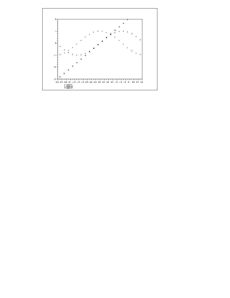
//captions for identifying the curves
//controlling the boundaries of the plot and the tics on axes
x=-%pi:0.3:%pi;
y1=sin(x);y2=cos(x);y3=x;
X=[x;x;x]; Y=[y1;y2;y3];
plot2d1("gnn",X',Y',[1 2 3]',"111","caption1@caption2@caption3",...
[-3,-3,3,2],[2,20,5,5]);
Figdirfigures/
For different plots the simple commands without any argument show a demo (e.g plot2d3() ).