The purpose of this appendix is to illustrate some of the more sophisticated aspects of Scilab by the way of an example. The example shows how Scilab can be used to symbolically represent the inter-connection of multiple systems which in turn can then be used to numerically evaluate the performance of the inter-connected systems. The symbolic representation of the inter-connected systems is done with a function called bloc2exp and the evaluation of the resulting system is done with evstr .
The example illustrates the symbolic inter-connection of the
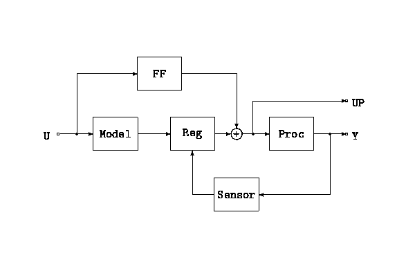
systems shown in Figure B.1.
The system illustrated in Figure B.1 can be represented in Scilab by using the function bloc2exp. The use of bloc2exp is illustrated in the following Scilab session. There a two kinds of objects: ``transfer'' and ``links''. The example considered here admits 5 transfers and 7 links. First the transfer are defined in a symbolic manner. Then links are defined and an ``interconnected system'' is defined as a specific list. The function bloc2exp evaluates symbolically the global transfer and evstr evaluates numerically the global transfer function once the systems are given ``values'', i.e. are defined as Scilab linear systems.
-->model=2;reg=3;proc=4;sensor=5;ff=6;somm=7;

-->tm=list('transfer','model');tr=list('transfer',['reg(:,1)','reg(:,2)']);

-->tp=list('transfer','proc');ts=list('transfer','s
ensor');

-->tf=list('transfer','ff');tsum=list('transfer',['1','1']);

-->lum=list('link','input',[-1],[model,1],[ff,1]);

-->lmr=list('link','model output',[model,1],[reg,1]);

-->lrs=list('link','regulator output',[reg,1],[somm,1]);

-->lfs=list('link','feed-forward output',[ff,1],[somm,2]);

-->lsp=list('link','proc input',[somm,1],[proc,1],[-2]);

-->lpy=list('link','proc output',[proc,1],[sensor,1],[-1]);

-->lsup=list('link','sensor output',[sensor,1],[reg,2]);

-->syst=...
 list('blocd',tm,tr,tp,ts,tf,tsum,lum,lmr,lrs,lfs,lsp,lpy,lsup);

-->[sysf,names]=bloc2exp(syst)
 names     =


       names>1

 input

       names>2

!proc output  !
!             !
!proc input   !
 sysf      =

!proc*((eye()-reg(:,2)*sensor*proc)\(-(-ff-reg(:,1)*model)))  !
!                                                           !
!(eye()-reg(:,2)*sensor*proc)\(-(-ff-reg(:,1)*model))         !
Note that the argument to bloc2exp is a list of lists. The
first element of the list syst is (actually) the character string
'blocd' which indicates that the list represents a block-diagram
inter-connection of systems. Each list entry in the list syst
represents a block or an inter-connection in Figure B.1.
The form of a list which represents a block begins with a character
string 'transfer' followed by a matrix of character strings
which gives the symbolic name of the block. If the block is multi-input
multi-output the matrix of character strings must be represented as
is illustrated by the block Reg.
The inter-connections between blocks is also represented by lists. The first element of the list is the character string 'link'. The second element of the inter-connection is its symbolic name. The third element of the inter-connection is the input to the connection. The remaining elements are all the outputs of the connection. Each input and output to an inter-connection is a vector which contains as its first element the block number (for instance the model block is assigned the number 2). The second element of the vector is the port number for the block (for the case of multi-input multi-output blocks). If an inter-connection is not attached to anything the value of the block number is negative (as for example the inter-connection labeled 'input' or is omitted.
The result of the bloc2exp function is a list of names which give the unassigned inputs and outputs of the system and the symbolic transfer function of the system given by sysf. The symbolic names in sysf can be associated to polynomials and evaluated using the function evstr. This is illustrated in the following Scilab session.
-->s=poly(0,'s');ff=1;sensor=1;model=1;proc=s/(s^2+3*s+2);

-->reg=[1/s 1/s];sys=evstr(sysf)
 sys       =

!     1 + s          !
!   ----------       !
!             2      !
!   1 + 3s + s       !
!                    !
!              2   3 !
!   2 + 5s + 4s + s  !
!   ---------------- !
!           2   3    !
!     s + 3s + s     !
The resulting polynomial transfer function links the input of the block system to the two outputs. Note that the output of evstr is the rational polynomial matrix sys whereas the output of bloc2exp is a matrix of character strings.
The symbolic evaluation which is given here is not very efficient with large interconnected systems. The function bloc2ss performs the previous calculation in state-space format. Each system is given now in state-space as a syslin list or simply as a gain (constant matrix). Note bloc2ss performs the necessary conversions if this is not done by the user. Each system must be given a value before bloc2ss is called. All the calculations are made in state-space representation even if the linear systems are given in transfer form.