Wiegner filter

//define system macro which generates the next
//observation given the old state
   deff('[x1,y]=system(x0,f,g,h,q,r)',[
        'rand(''normal'');'
        'q2=chol(q);'
        'r2=chol(r);'
        'u=q2''*rand(ones(x0));'
        'v=r2''*rand(ones(x0));'
        'x1=f*x0+g*u;'
        'y=h*x1+v;'])
//initialize state statistics (mean and error variance)
   m0=[10;10];
   p0=[100 0;0 100];
//create system
   f=[1.15 .1;0 .8];
   g=[1 0;0 1];
   h=[1 0;0 1];
   [hi,hj]=size(h);
//noise statistics
   q=[.01 0;0 .01];
   r=20*eye(2,2);
//initialize system process
   rand('seed',66),
   rand('normal'),
   p0c=chol(p0);
   x0=m0+p0c'*rand(ones(m0));
   y=h*x0+chol(r)'*rand(ones(1:hi))';
   yt=y;
//initialize plotted variables
   x=x0; ft=f; gt=g; ht=h; qt=q; rt=r;
   n=10;
   for k=1:n,
//generate the state and observation at time k (i.e. xk and yk)
      [x1,y]=system(x0,f,g,h,q,r);
      x=[x x1];x0=x1;
      yt=[yt y];ft=[ft f];gt=[gt g];ht=[ht h];qt=[qt q];rt=[rt r];
   end,
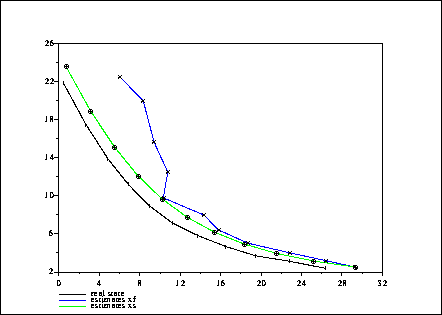
//get the wiener filter estimate
   [xs,ps,xf,pf]=wiener(yt,m0,p0,ft,gt,ht,qt,rt);
//plot result
//plot frame, real state (x), and estimates (xf, and xs)
   plot2d([x(1,:)',xf(1,:)',xs(1,:)'],..
          [x(2,:)',xf(2,:)',xs(2,:)'],[1 2 3],"161",..
          'real state@estimates xf@estimates xs'),
//mark data points (* for real data, o for estimates)
    plot2d([x(1,:)',xf(1,:)',xs(1,:)'],..
          [x(2,:)',xf(2,:)',xs(2,:)'],-[1 2 3],"000",..
          'real state@estimates xf@estimates xs'),