Delta Method implementation to estimate standard errors in a {tidyverse} workflow.
You can install the development version of tidydelta from GitHub with:
remotes::install_github("JavierMtzRdz/tidydelta")
# Or
devtools::install_github("JavierMtzRdz/tidydelta") In general terms, the Delta Method provides a tool for approximating the behaviour of an estimator \(\phi(T_n)\) using Taylor Expansion, where \(T_n\) is an estimator of a parameter \(\theta\), and \(\phi\) is a function. To derive this result, we should begin with the observation that, according to the continuous mapping theorem, if \(T_n \xrightarrow{\mathbb{P}} \theta\) implies \(\phi(T_n) \xrightarrow{\mathbb{P}} \phi(\theta)\) assuming that \(\phi\) is a continuous function (Vaart 2000, 25).
This observation allows us to take a step forward to decompose the theorem of the DM. Assuming that \(\phi\) is not only continuous but also differentiable and further assuming that \(\sqrt{n} (T_n - \theta)\) converges in distribution to a variable \(T\) as the sample size \(n\) increases, (Bouchard-Côté n.d., 87) we can employ Taylor Expansion to show that
\[ \sqrt{n} (\phi(T_n) - \phi(\theta)) \approx \phi'(\theta)\sqrt{n} (T_n - \theta). \]
Now, as the sample size \(n\) becomes larger, the expression \(\sqrt{n} (\phi(T_n) - \phi(\theta))\) converges in distribution to \(\phi'(\theta)T\) (Vaart 2000, 25; Bouchard-Côté n.d.).
Given the previous result, we can rearrange the equations to show that
\[ \sqrt{n} (\phi(T_n) - \phi(\theta)) \sim N(0, \phi'(\theta)^2\sigma^2) \]
as \(n\) grows larger. For this reason, it is not a surprise that one of the primary uses of the Delta Method is to approximate the variance of transformations of estimators.
We often encounter scenarios where our \(\theta\) can be expressed as a function of more than one parameter. For instance, we may be interested in the transformation \(\phi\) of \(\theta = (\theta_1, \ldots, \theta_k)\) (Zepeda-Tello et al. 2022). In this case, we are dealing with a multivariate parameter space and the estimator \(T_{n,k} = (Y_{n,1}, \ldots, Y_{n,k})\) becomes a random vector. Consequently, the asymptotic behaviour of the estimator \(T_{n,k}\) can be seen as follows (Weisberg 2005, 79–80)
\[ \sqrt{n} (T_{n,k} - \theta) \leadsto N(0, \Sigma). \]
To approximate this scenario using the Delta Method, we need to compute the vector of all partial derivatives of \(\phi(\theta)\) with respect to each parameter \(\theta_1, \ldots, \theta_k\). This vector is denoted as \(\nabla \phi\). With this vector, we can extend the Delta Method to the multivariate case stating that asymptotically
\[ \sqrt{n} (\phi(T_{n,k}) - \phi(\theta)) \leadsto N(0, \nabla_{\theta}^\top\Sigma \nabla_{\theta}). \]
In this equation, \(\nabla_{\theta}^\top\) represents the transpose of the gradient vector \(\nabla \phi\), and \(\Sigma\) is the covariance matrix of the random vector \(T_{nk}\) (Weisberg 2005, 79–80).From this, we obtain that \(se(\theta) = \sqrt{\nabla_{\theta}^\top\Sigma \nabla_{\theta}}\), which constitutes the function that is being implemented in this project.
Using tidydelta(), the following commands are equivalent:
# Load packages
library(tidydelta)
library(tidyverse)

# Simulate samples
set.seed(547)
x <- rnorm(10000, mean = 5, sd = 2)
y <- rnorm(10000, mean = 15, sd = 3)

bd <- tibble(x, y)

# Equivalent uses of tidydelta()
tidydelta(~ y / x,
  conf_lev = .95
)
#> # A tibble: 1 × 6
#>       y     x   T_n    se lower_ci upper_ci
#>   <dbl> <dbl> <dbl> <dbl>    <dbl>    <dbl>
#> 1  15.0  5.02  2.99  1.33    0.378     5.61

tidydelta(~ bd$y / bd$x,
  conf_lev = .95
)
#> # A tibble: 1 × 6
#>       y     x   T_n    se lower_ci upper_ci
#>   <dbl> <dbl> <dbl> <dbl>    <dbl>    <dbl>
#> 1  15.0  5.02  2.99  1.33    0.378     5.61
bd %>%
  summarise(tidydelta(~ y / x,
    conf_lev = .95
  ))
#> # A tibble: 1 × 6
#>       y     x   T_n    se lower_ci upper_ci
#>   <dbl> <dbl> <dbl> <dbl>    <dbl>    <dbl>
#> 1  15.0  5.02  2.99  1.33    0.378     5.61
Now, the data frame is divided into samples to compare the
transformation of the sample with the estimation of
tidydelta(). In the real world, you would not need to
compute the Delta Method if you have many samples, but it shows how it
can be incorporated in a workflow with tidyverse.
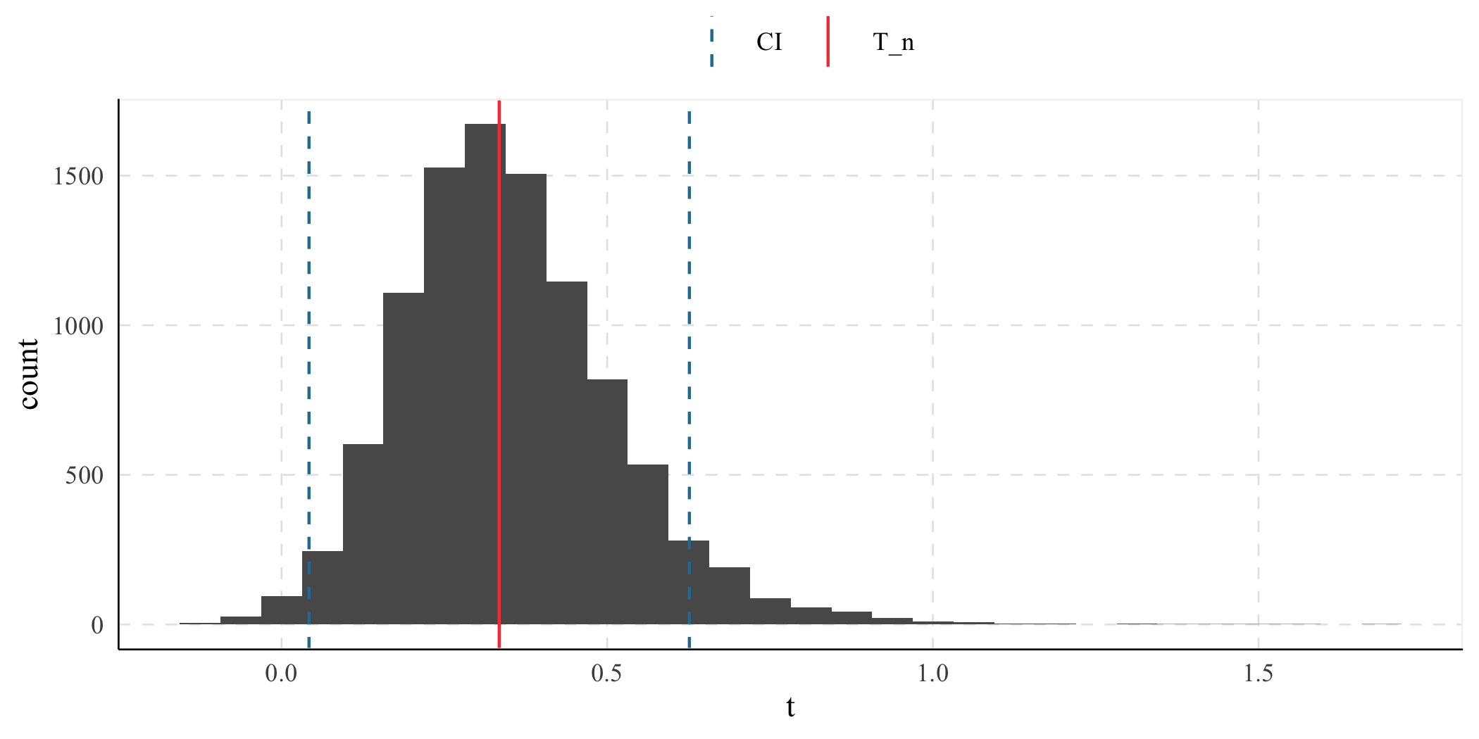
(result <- bd %>%
  summarise(tidydelta(~ x / y,
    conf_lev = .95
  )))
#> # A tibble: 1 × 6
#>       x     y   T_n    se lower_ci upper_ci
#>   <dbl> <dbl> <dbl> <dbl>    <dbl>    <dbl>
#> 1  5.02  15.0 0.334 0.149   0.0422    0.626

ggplot() +
  geom_histogram(
    data = bd %>%
      mutate(t = x / y),
    aes(x = t)
  ) +
  geom_vline(aes(
    xintercept = result$T_n,
    color = "T_n"
  )) +
  geom_vline(
    aes(
      xintercept = c(
        result$lower_ci,
        result$upper_ci
      ),
      color = "CI"
    ),
    linetype = "dashed"
  ) +
  labs(color = element_blank())