The goal of sfislands is to make it easier to deal with
geographic datasets which contain islands. It does so using a tidy
framework in the spirit of Josiah Parry’s sfdep package.
Such a situation can lead to two issues.
Firstly, if unaddressed, the presence of such islands or exclaves can make certain types of contiguity-based modelling impossible.
Secondly, just because two areas are separated by, say, a body of water, this does not necessarily mean that they are to be considered independent of each other.
This package offers solutions to allow for the inclusion or exclusion of these units within an uncomplicated workflow.
A pre-print of a paper discussing the package is available here.
Install the released version from CRAN:
install.packages("sfislands")You can install the development version of sfislands
from GitHub
with:
# install.packages("devtools")
devtools::install_github("horankev/sfislands")The initial setting-up of neighbourhood structures can be frustrating for people who are eager to get started with fitting spatial models. This is especially so when the presence of discontiguities within a geographical dataset means that, even having set up a neighbours list, the model will still not run without further awkward data manipulations.
As an aid to setting up neighbourhood structures, particularly
when islands are involved, the package has a function to quickly map any
neighbourhood structure for visual inspection. This can also be used to
examine the output of sfdep neighbour functions. Such maps
can be used to check if the structure makes sense, given the
researcher’s knowledge about the geography of the study area.
If some units have been assigned as neighbours inappropriately, or if we wish to add additional connections, there are functions to allow this to be done in a straightforward and openly reportable way.
Once an appropriate neighbourhood structure is in place,
different types of statistical tests and models can be performed.
sfdep contains functionality to perform such tests, and the
output from sfislands can be used in its
functions.
The contiguity outputs from sfislands can be
directly used to fit different types of (multilevel) (I)CAR models
using, for example, the mgcv, brms,
stan or INLA packages.
For mgcv in particular, the predictions of such
models can be quite tedious to extract and visualise.
sfislands can streamline this workflow from the human side.
Furthermore, there is a function to draw maps of these predictions for
quick inspection.
The following is a brief explanations of the functions contained in
the sfislands package and a workflow within which they
could be used.
The first group can be seen as pre-functions, designed to create a neighbourhood structure suitable for certain types of models.
Once a model has been fit (using mgcv in this case), the
post-functions can be used to extract the predictions.
| function: | purpose: |
|---|---|
| st_bridges() | Create a neighbours list, matrix, or sf dataframe
containing a neighbours list or matrix as column “nb”, while accounting
for islands. |
| st_quickmap_nb() | Check contiguities visually on map. |
| st_check_islands() | Check assignment of island contiguities in a dataframe. |
| st_force_join_nb() | Enforce changes to any connections. |
| st_force_cut_nb() | Enforce changes to any connections. |
Use the output of st_bridges() as both the data and
neighbourhood inputs for a model using, for example, mgcv,
brms or inla.
| function: | purpose: |
|---|---|
| st_augment() | Augment the original dataframe with model predictions. |
| st_quickmap_preds() | Generate quick maps of these predictions. |
The dataset uk_elections, which is provided with the
package, is used for the following demonstrations. It is an
sf dataset with geometries for each of the 632 Westminster
parliamentary constituencies of England, Scotland and Wales in the 2019
general election. For each constituency, it contains socio-economic data
from the 2011 census. It also shows the Butler swing between
the 2017 and 2019 elections, which is a measure of the change in voter
allegiance in favour of the Conservative Party from the Labour
Party.
To demonstrate the st_bridges() function for preparing
an adjacency matrix, we focus on Scotland. It is the nation with the
highest number of islands. The function, with default arguments, returns
a dataframe with an additional column named nb. This column
is a named neighbourhood list of class nb. The default
neighbourhood structure which it computes is:
for constituencies which are not islands, first-order queen contiguity. A constituency is considered to be a neighbour of all of those with which it shares at least a vortex.
for islands, contiguities are assigned to the
two nearest constituencies to each island. This number can be altered
using the link_islands_k argument.
scotland_df <- uk_election |> filter(country == "Scotland")
nbsf <- st_bridges(df = scotland_df,
                   row_identifier = "constituency_name",
                   link_islands_k = 2)
This new dataframe has the following form (with a column named
nb containing a neighbours list):
head(nbsf)
#> Simple feature collection with 6 features and 10 fields
#> Geometry type: GEOMETRY
#> Dimension:     XY
#> Bounding box:  xmin: 92527.68 ymin: 571251.1 xmax: 397261.7 ymax: 812377.5
#> Projected CRS: OSGB36 / British National Grid
#>   degree_educated health_not_good     white  con_swing population   region
#> 1       0.2659346      -0.8699365 0.1441816  7.1285493      99654 Scotland
#> 2       1.6283752      -1.7731408 0.3038995  2.9732599      93197 Scotland
#> 3      -1.3538678       0.8155333 0.6963927 -0.2362672      85845 Scotland
#> 4      -0.6852759      -0.6765349 0.7250742  1.7350840      86004 Scotland
#> 5       0.2535023      -0.3624242 0.7174423  3.9062703      88166 Scotland
#> 6      -0.6898382       0.6590625 0.7272781  4.4404142      93308 Scotland
#>     county        constituency_name  country                     nb
#> 1 Scotland           Aberdeen North Scotland              2, 36, 58
#> 2 Scotland           Aberdeen South Scotland                  1, 58
#> 3 Scotland       Airdrie and Shotts Scotland 11, 12, 41, 42, 43, 46
#> 4 Scotland                    Angus Scotland         15, 16, 54, 58
#> 5 Scotland          Argyll and Bute Scotland         54, 55, 57, 59
#> 6 Scotland Ayr, Carrick and Cumnock Scotland         10, 13, 14, 39
#>                         geometry
#> 1 MULTIPOLYGON (((395379.7 80...
#> 2 POLYGON ((396214 805849.7, ...
#> 3 POLYGON ((290854.4 662154.9...
#> 4 POLYGON ((374164.5 762668.6...
#> 5 MULTIPOLYGON (((139257.4 64...
#> 6 MULTIPOLYGON (((246939 6250...
We can inspect (and openly report) what additional contiguities have
been added to the standard queen contiguity structure using the function
st_check_islands().
st_check_islands(nbsf)
#>           island_names island_num nb_num                              nb_names
#> 1 Na h-Eileanan An Iar         47      9 Caithness, Sutherland and Easter Ross
#> 2 Na h-Eileanan An Iar         47     51                   Orkney and Shetland
#> 3 Na h-Eileanan An Iar         47     55               Ross, Skye and Lochaber
#> 4  Orkney and Shetland         51      9 Caithness, Sutherland and Easter Ross
#> 5  Orkney and Shetland         51     47                  Na h-Eileanan An Iar
The overall contiguity structure can be visualised using the function
st_quickmap_nb(), whose output is shown below on the
left.
ggarrange(
  st_quickmap_nb(nbsf),

  st_quickmap_nb(nbsf,
                 concavehull = TRUE,
                 nodes = "numeric",
                 numericsize = 3.5),

  ncol = 2
)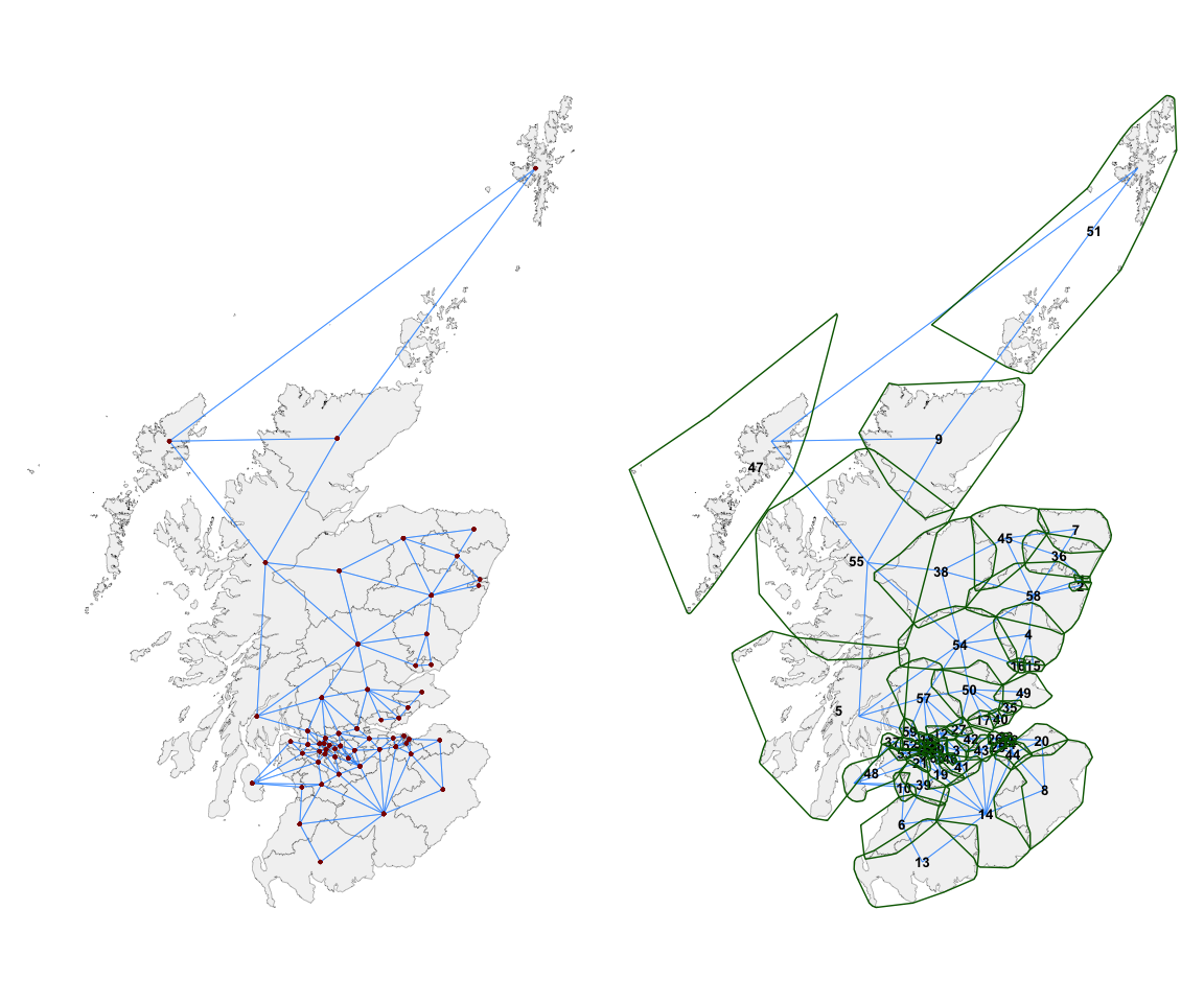
However, it is often the case that each island unit (in this
case, constituency) is in fact a multipolygon of islands. To make this
clearer, the argument concavehull = TRUE can be chosen.
These green boundaries (shown above on the right) around each
constituency are for reference purpose only and do not influence the
assignment of contiguities. They show which group of islands
are considered as one constituency of islands. Furthermore, the
argument nodes = "numeric" represents the centroids of each
unit with its index number instead of a geometric point. This can be
useful for editing the adjacencies, particularly if the researcher is
not familiar with the names of the individual spatial units.
A researcher can now use domain knowledge or a particular hypothesis
to edit these contiguities. For instance, we may not be happy with the
connection between 47 (Na h-Eileanan An Iar) and 51 (Orkney and
Shetland) and wish to remove it. We might instead feel that it is
important for 47 and 5 to be considered neighbours. This can be easily
achieved, as shown below, using the st_force_cut_nb() and
st_force_join_nb() functions. The spatial units whose
relationships we wish to change can be referenced by name or by index
number.
nbsf <- st_bridges(df = uk_election |> filter(country == "Scotland"),
                   row_identifier = "constituency_name",
                   link_islands_k = 2) |>
  st_force_cut_nb("Na h-Eileanan An Iar", "Orkney and Shetland") |>
  st_force_join_nb(47, 5)
The results of these changes as visualised in map form are shown below:
ggarrange(
  st_quickmap_nb(nbsf,
                 concavehull = TRUE,
                 nodes = "numeric",
                 numericsize = 3.5),

  st_quickmap_nb(nbsf),

  ncol = 2
)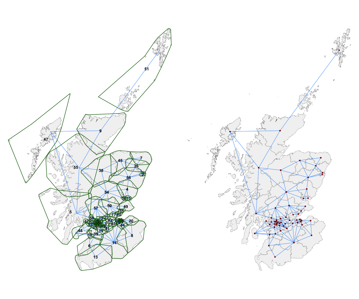
The above process can be iterated until we are happy that the structure conforms with our hypothesis of connectivity within the study area.
Having set up a neighbourhood structure and embedded it as a named
list or matrix within the original sf dataset as a column
named nb, the workflow to generate and visualise
predictions from a model (in this case using mgcv) is very
straightforward and consists of only 3-4 lines of code.
For example, we can use the mgcv package to generate
quite a complicated model with various random intercepts and slopes at
region and county level, and additionally, different Markov Random Field
ICAR smooths at the constituency level. This is done very quickly by
st_bridges() to prepare the data,mgcv::gam() formulation, and
thenst_augment() function.This gives the following output, with all of the spatially varying predictions and their standard errors being added as extra columns before the final geometry column:
prep_data <- st_bridges(uk_election, "constituency_name") # decide upon the contiguities and add them to the df

model1 <- gam(con_swing ~
               s(region, bs="re") + # region level random intercept
               s(county, bs="re") + # county level random intercept
               s(county, degree_educated, bs="re") + # county level random coefficient
               s(constituency_name, bs='mrf',
                 xt=list(nb=prep_data$nb),k=10) + # ICAR constituency ICAR varying coefficients
               s(constituency_name, by=white, bs='mrf',
                 xt=list(nb=prep_data$nb),k=10), # ICAR constituency ICAR varying coefficients
             data=prep_data, method="REML") |>  # pipe into function to get estimates
  st_augment(prep_data)

head(model1)
#> Simple feature collection with 6 features and 20 fields
#> Geometry type: GEOMETRY
#> Dimension:     XY
#> Bounding box:  xmin: 264110.4 ymin: 148666.1 xmax: 488768.5 ymax: 812377.5
#> Projected CRS: OSGB36 / British National Grid
#>   degree_educated health_not_good      white  con_swing population     region
#> 1     -1.21794372       2.4694480  0.6393329  8.5917223      66133      Wales
#> 2      0.04609836       0.5666903  0.6561204  2.2040312      56415      Wales
#> 3      0.26593462      -0.8699365  0.1441816  7.1285493      99654   Scotland
#> 4      1.62837520      -1.7731408  0.3038995  2.9732599      93197   Scotland
#> 5     -1.35386780       0.8155333  0.6963927 -0.2362672      85845   Scotland
#> 6     -0.21109416      -1.3619136 -0.1675498  5.6993250     103922 South East
#>           county  constituency_name  country                           nb
#> 1 West Glamorgan           Aberavon    Wales  80, 157, 371, 419, 451, 547
#> 2          Clwyd          Aberconwy    Wales                 12, 141, 181
#> 3       Scotland     Aberdeen North Scotland                  4, 239, 595
#> 4       Scotland     Aberdeen South Scotland                       3, 595
#> 5       Scotland Airdrie and Shotts Scotland 142, 156, 309, 327, 332, 369
#> 6      Hampshire          Aldershot  England            70, 395, 517, 544
#>   random.effect.region random.effect.county
#> 1           0.07736634           -0.0889861
#> 2           0.07736634           -0.1062061
#> 3          -1.69257542           -0.2986088
#> 4          -1.69257542           -0.2986088
#> 5          -1.69257542           -0.2986088
#> 6          -0.60617303            0.2472990
#>   random.effect.degree_educated|county mrf.smooth.constituency_name
#> 1                           -3.0504238                   0.08001029
#> 2                           -1.6077523                   0.10070833
#> 3                           -0.1165337                  -0.30112582
#> 4                           -0.1165337                  -0.30111510
#> 5                           -0.1165337                  -0.34218741
#> 6                           -2.0453936                   0.01698329
#>   mrf.smooth.white|constituency_name se.random.effect.region
#> 1                          0.9971918               0.5881627
#> 2                          1.2785329               0.5881627
#> 3                          1.2800763               0.6985112
#> 4                          1.2799615               0.6985112
#> 5                          1.7736548               0.6985112
#> 6                         -0.1353957               0.5113682
#>   se.random.effect.county se.random.effect.degree_educated|county
#> 1               0.4400444                               1.0549478
#> 2               0.4432314                               1.7152822
#> 3               0.4500975                               0.2933430
#> 4               0.4500975                               0.2933430
#> 5               0.4500975                               0.2933430
#> 6               0.3825063                               0.6696364
#>   se.mrf.smooth.constituency_name se.mrf.smooth.white|constituency_name
#> 1                       0.3101948                             0.7308175
#> 2                       0.2039813                             0.4377840
#> 3                       0.5769227                             1.0462122
#> 4                       0.5769674                             1.0463117
#> 5                       0.4265664                             0.7384490
#> 6                       0.1762707                             0.2423523
#>                         geometry
#> 1 POLYGON ((290786.3 202886.7...
#> 2 POLYGON ((283209.3 381440.5...
#> 3 MULTIPOLYGON (((395379.7 80...
#> 4 POLYGON ((396214 805849.7, ...
#> 5 POLYGON ((290854.4 662154.9...
#> 6 POLYGON ((485408.1 159918.6...
The predictions can be quickly visualised using
st_quickmap_preds(). As this function generates a list of
ggplots, they can be conveniently visualised using the
ggarrange() function from the ggpubr
package.
plots <- st_quickmap_preds(model1)
ggarrange(plotlist = plots, legend = "none", nrow=1)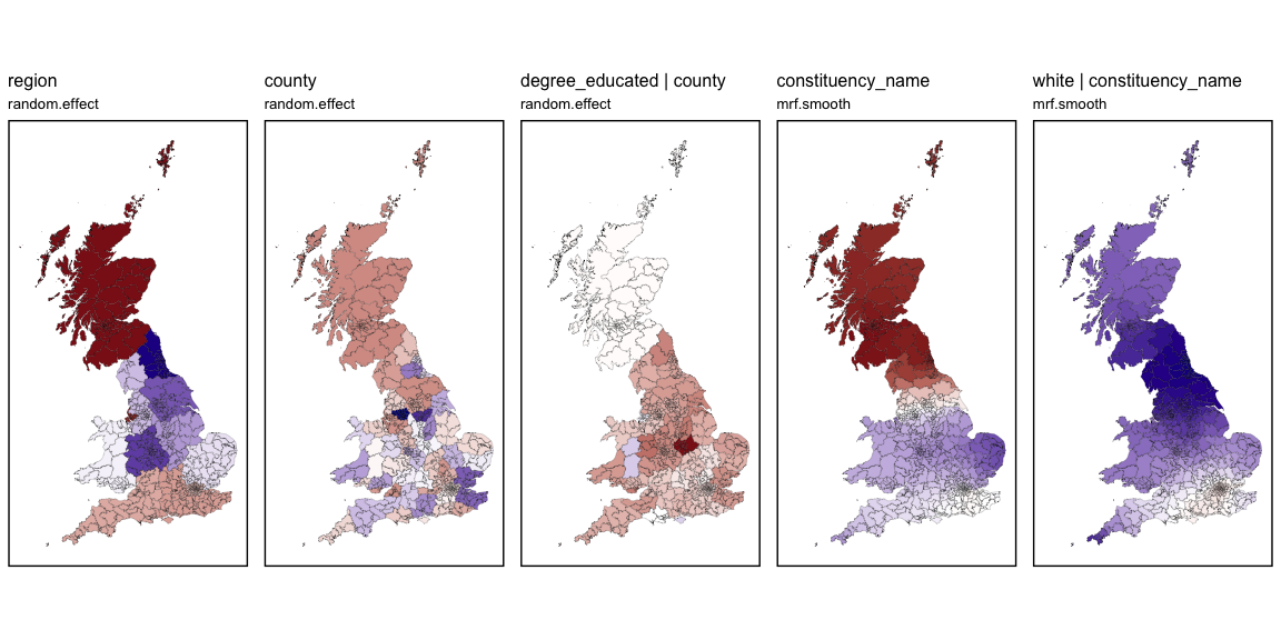
To emphasise the simplicity of the process, the a modified version of
the following sequence of commands will generate a series of plots of
all of the spatially varying elements of a model defined in
mgcv:
prep_data <- st_bridges(...)

gam(..., data = prep_data) |>
  st_augment() |>
  st_quickmap_preds()
It is also possible to conduct the same kind of augmenting and
plotting of models generated using the lme4 and
nlme packages.
Further information and vignettes containing more detailed examples are available here.