![]()
![]()
![]()
In ancient Roman mythology, Pluto was the ruler of
the underworld and presides over the afterlife.
Pluto was frequently conflated with
Plutus, the god of wealth, because mineral wealth was found
underground.
When plotting with R, you try once, twice, practice again and again, and finally you get a pretty figure you want.
It’s a plot tour, a tour about repetition and
reward.
Hope plutor helps you on the tour!
You can install the development version of plutor like
so:
devtools::install_github("william-swl/plutor")And load the package:
library(plutor)It is recommended to perform initialization, which adjusts the
default plotting parameters in an interactive environment (such as
jupyter notebook) and sets the default theme to
theme_pl().
pl_init()Description values plot:
The describe geom is used to create description values plot, including center symbol and error symbol.
The center symbol can be mean, median or other custom functions.
The error symbol can be sd, quantile or other custom functions.
mini_diamond %>% ggplot(aes(x = cut, y = price)) +
  geom_point() +
  geom_describe()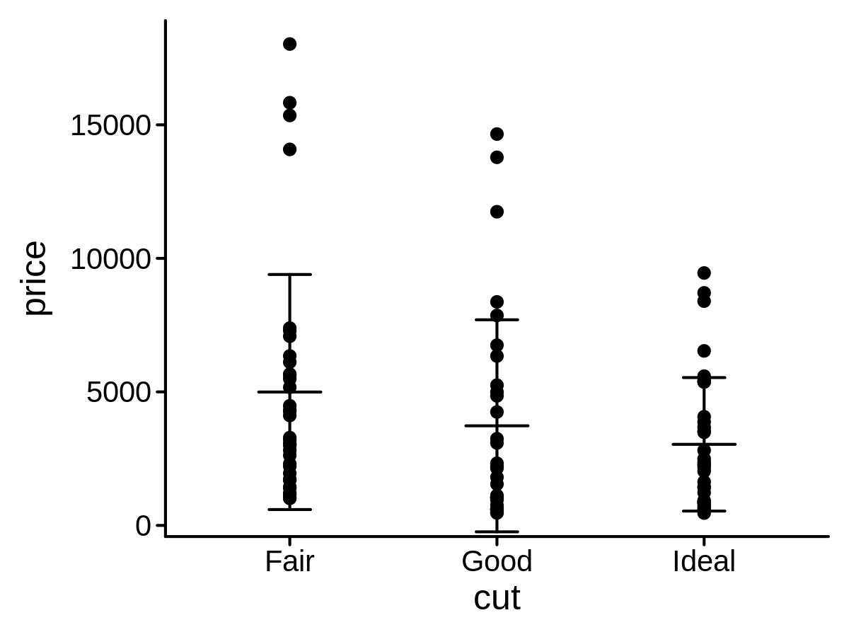
center_func <- median
low_func <- function(x, na.rm) {
  quantile(x, 0.25, na.rm = na.rm)
}

high_func <- function(x, na.rm) {
  quantile(x, 0.75, na.rm = na.rm)
}

mini_diamond %>% ggplot(aes(x = cut, y = price)) +
  geom_point() +
  geom_describe(center_func = center_func, low_func = low_func, high_func = high_func)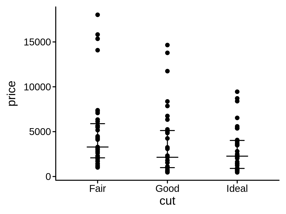
Add p value and fold change on a plot
p <- ggplot(data = mini_diamond, mapping = aes(x = cut, y = price)) +
  geom_point() +
  geom_compare(cp_label = c("psymbol", "right_deno_fc"), lab_pos = 25000, step_increase = 0.3) +
  ylim(0, 40000)
p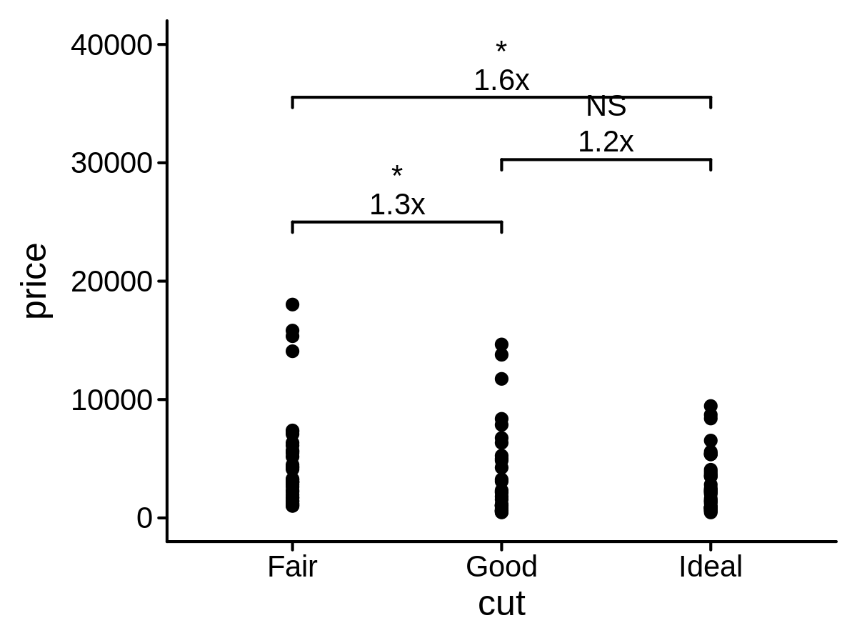
ggplot(data = mini_diamond, mapping = aes(x = cut, y = price)) +
  geom_point() +
  geom_compare(cp_ref = "Good", cp_inline = TRUE, lab_pos = 22000, brackets_widen = 0.1) +
  geom_compare(cp_ref = "Ideal", cp_inline = TRUE, lab_pos = 25000, brackets_widen = 0.1) +
  ylim(0, 40000)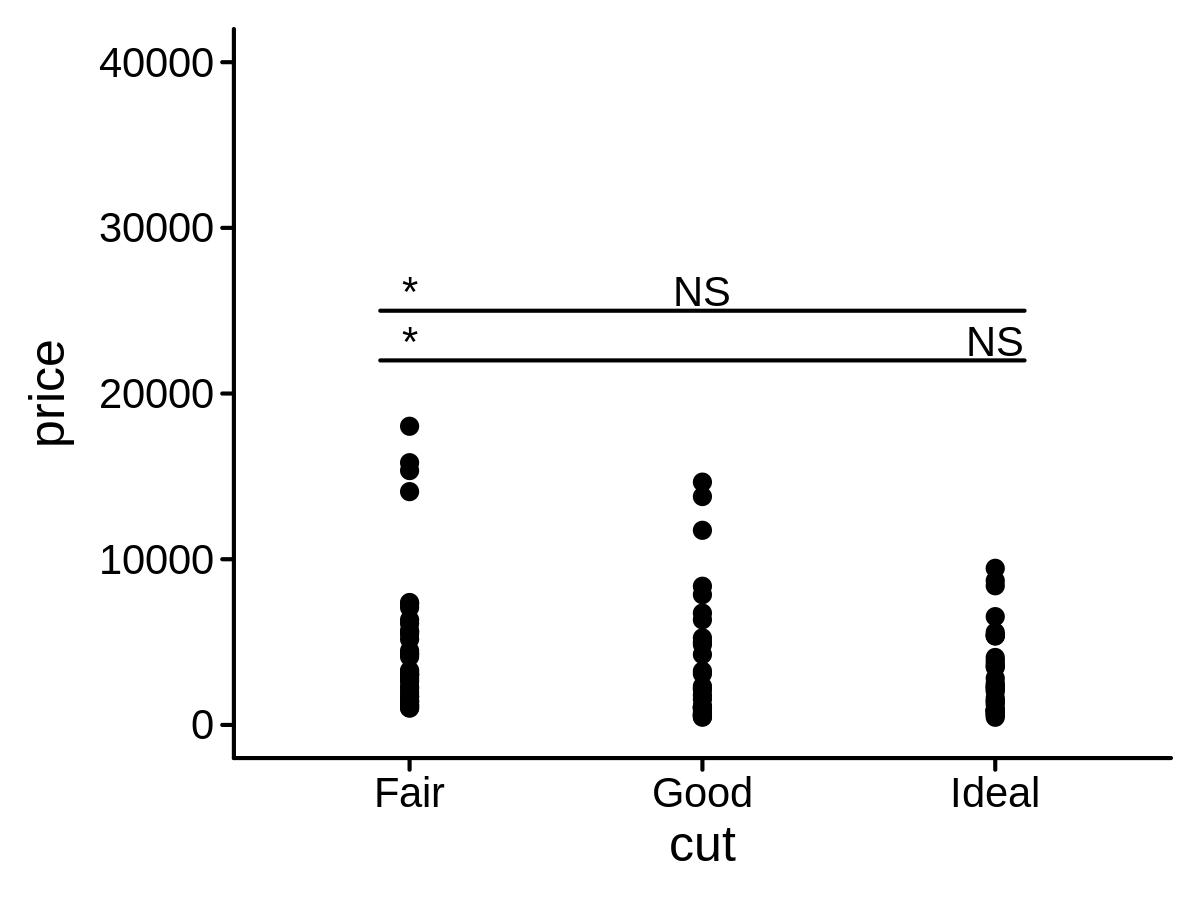
extract the result of geom_compare from a
ggplot object
head(extract_compare(p))
#>   PANEL x xend n1 n2     p plim psymbol       y1       y2       fc
#> 1     1 1    2 35 31 0.041 0.05       * 4995.057 3730.387 1.339018
#> 2     1 2    3 31 34  0.93 1.01      NS 3730.387 3036.588 1.228480
#> 3     1 1    3 35 34 0.018 0.05       * 4995.057 3036.588 1.644957
#>   right_deno_fc left_deno_fc    label cp_step       y    yend group
#> 1          1.3x        0.75x  *\n1.3x       0 25000.0 25000.0     1
#> 2          1.2x        0.81x NS\n1.2x       1 30269.2 30269.2     1
#> 3          1.6x        0.61x  *\n1.6x       2 35538.4 35538.4     1
A new Stat class to add mean labels on a plot
mini_diamond %>% ggplot(aes(x = cut, y = price)) +
  geom_point() +
  geom_text(aes(label = price), stat = "meanPL")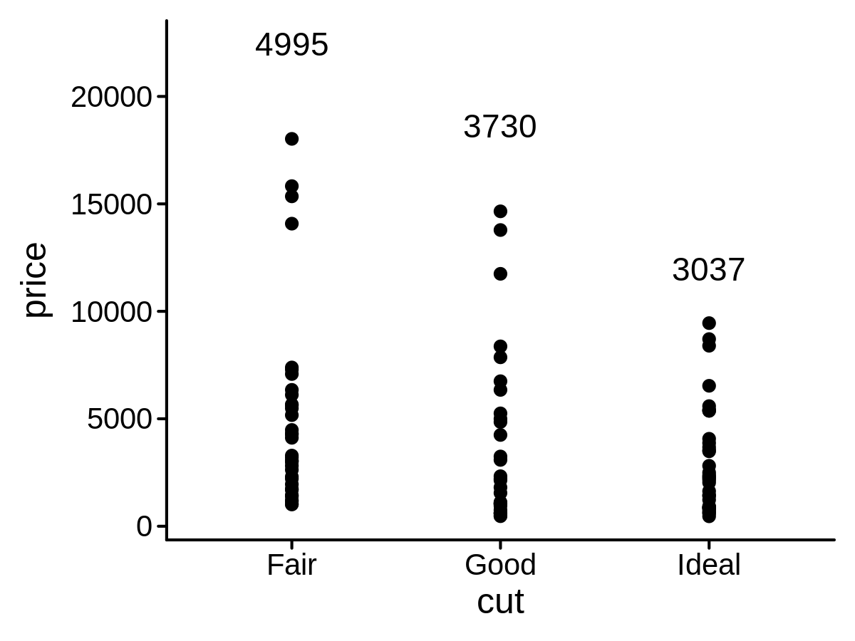
A new Stat class to add count labels on a plot
mini_diamond %>% ggplot(aes(x = cut, y = price)) +
  geom_point() +
  geom_text(aes(label = price), stat = "countPL")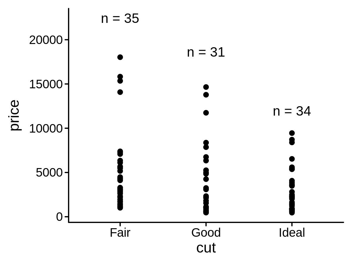
A new Stat class to add custom function labels on a
plot
lab_func <- function(x) {
  str_glue("mean = {round(mean(x))}\nn = {length(x)}")
}

mini_diamond %>% ggplot(aes(y = cut, x = price)) +
  geom_point() +
  geom_text(aes(label = price),
    stat = "funcPL",
    lab_func = lab_func, lab_pos = 25000
  ) +
  xlim(0, 30000)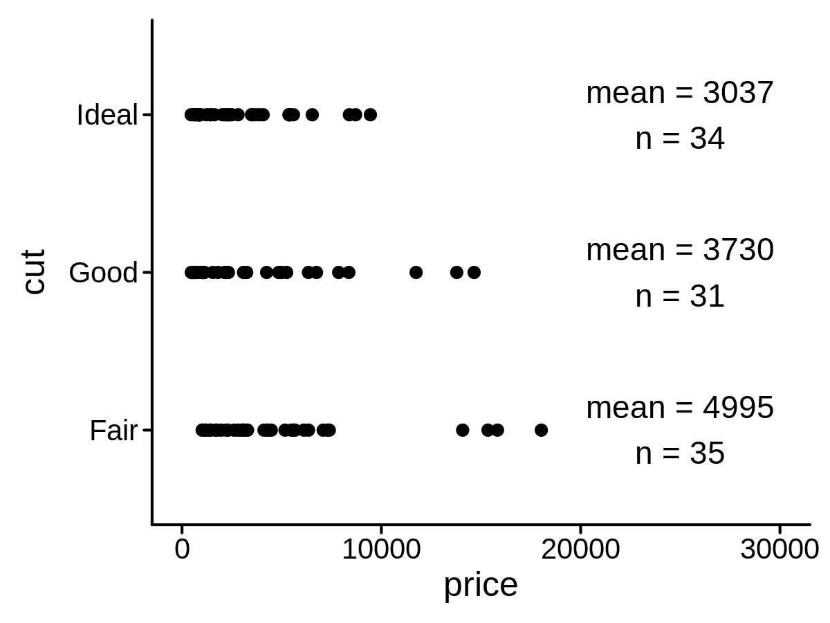
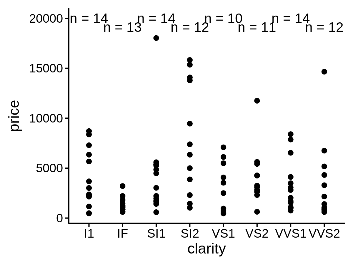
A new Position function to create float x/y position
mini_diamond %>% ggplot(aes(x = clarity, y = price)) +
  geom_point() +
  geom_text(aes(label = price),
    stat = "countPL",
    lab_pos = 20000, position = position_floatyPL()
  )
A variant of scale_y_log10() to show axis minor breaks
and better axis labels
mini_diamond %>% ggplot(aes(x = cut, y = price)) +
  geom_point() +
  geom_text(stat = "meanPL", lab_pos = 30000) +
  scale_y_log10_pl(show_minor_breaks = TRUE, limits = c(100, 100000))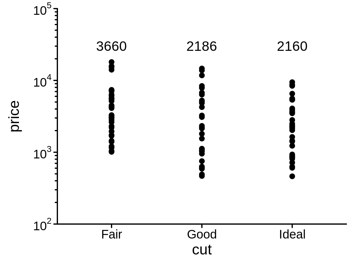
A variant of scale_y_continuous() to show axis minor
breaks
mini_diamond %>% ggplot(aes(x = cut, y = price)) +
  geom_point() +
  geom_text(stat = "meanPL", lab_pos = 25000) +
  scale_y_continuous_pl(limits = c(0, 40000), minor_break_step = 2500)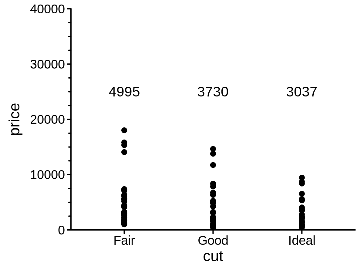
gradient_colors(c("blue", "red"), 10)
#>  [1] "#0000FF" "#1C00E2" "#3800C6" "#5500AA" "#71008D" "#8D0071" "#AA0055"
#> [8] "#C60038" "#E2001C" "#FF0000"plot_colors(gradient_colors(c("blue", "red"), 10))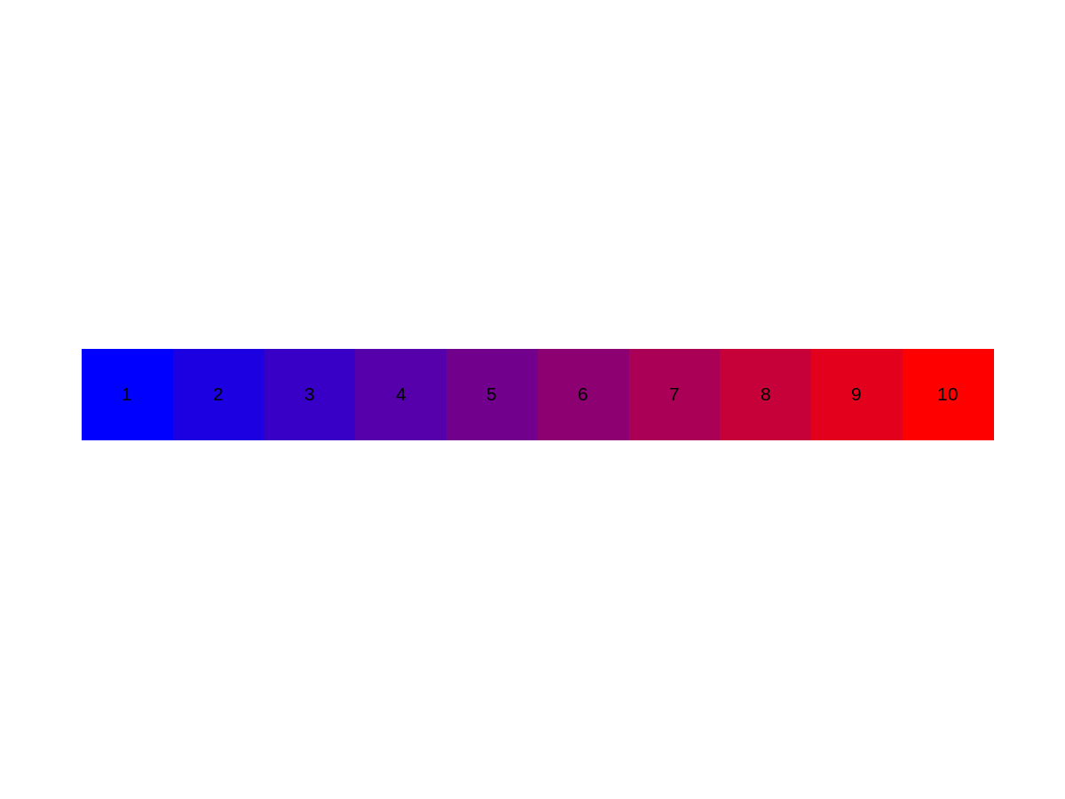
RColorBrewer package presetsbrewer_colors("Blues", 5) %>% plot_colors()
ggsci package presetssci_colors("npg", 5) %>% plot_colors()
scale_color_identity()assign_colors(mini_diamond, cut, colors = sci_colors("nejm", 8))
#> # A tibble: 100 × 8
#> id carat cut clarity price x y assigned_colors
#> <chr> <dbl> <chr> <chr> <int> <dbl> <dbl> <chr>
#> 1 id-1 1.02 Fair SI1 3027 6.25 6.18 #BC3C29FF
#> 2 id-2 1.51 Good VS2 11746 7.27 7.18 #0072B5FF
#> 3 id-3 0.52 Ideal VVS1 2029 5.15 5.18 #E18727FF
#> 4 id-4 1.54 Ideal SI2 9452 7.43 7.45 #E18727FF
#> 5 id-5 0.72 Ideal VS1 2498 5.73 5.77 #E18727FF
#> 6 id-6 2.02 Fair SI2 14080 8.33 8.37 #BC3C29FF
#> 7 id-7 0.27 Good VVS1 752 4.1 4.07 #0072B5FF
#> 8 id-8 0.51 Good SI2 1029 5.05 5.08 #0072B5FF
#> 9 id-9 1.01 Ideal SI1 5590 6.43 6.4 #E18727FF
#> 10 id-10 0.7 Fair VVS1 1691 5.56 5.41 #BC3C29FF
#> # … with 90 more rows# bioletter_colorsggplot(mini_diamond, aes(x = x, y = y, color = clarity)) +
geom_point(size = 2) +
facet_grid(. ~ cut) +
labs(title = "title", tag = "tag", caption = "caption") +
theme_pl()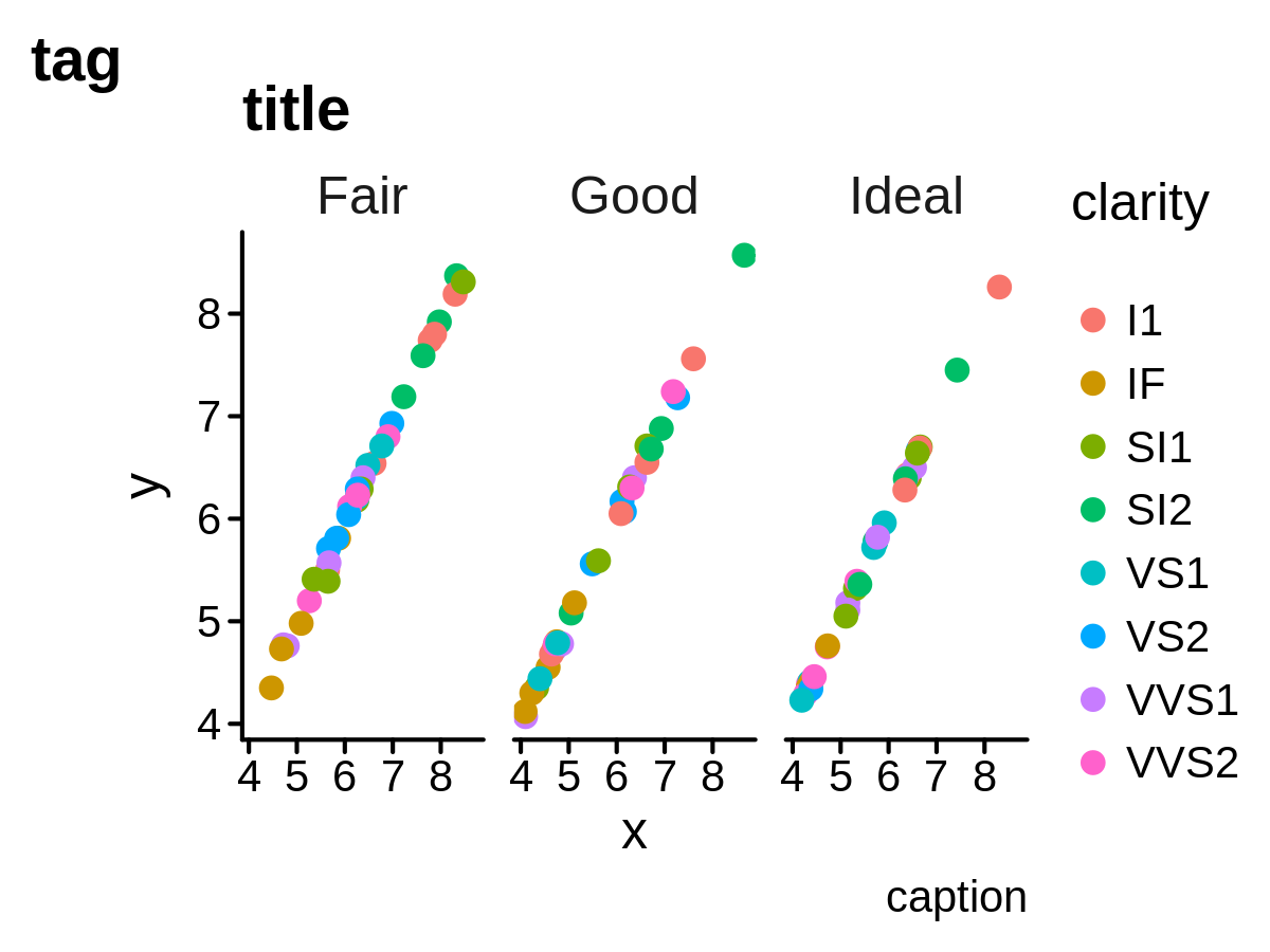
ggplot(mini_diamond, aes(x = x, y = y, color = clarity)) +
  geom_point(size = 2) +
  facet_grid(. ~ cut) +
  labs(title = "title", tag = "tag", caption = "caption") +
  theme_pl0()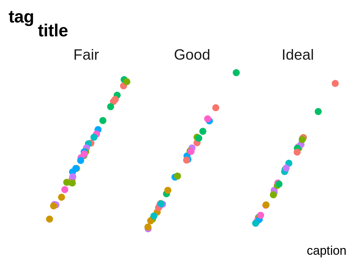
geom_xxx to unit
pt under 300 dpi# for text and points
# geom_point(..., size = ppt(5))
# geom_text(..., size = tpt(5))
# for lines
# geom_line(..., linewidth = lpt(1))pl_size(w = 4, h = 3, res = 300)# inches <-> centimeters
inch2cm(1)
#> [1] 2.54
#> attr(,"unit")
#> [1] 1
in2cm(1)
#> [1] 2.54
#> attr(,"unit")
#> [1] 1
cm2inch(1)
#> [1] 0.3937008
#> attr(,"unit")
#> [1] 2
cm2in(1)
#> [1] 0.3937008
#> attr(,"unit")
#> [1] 2
# inches <-> millimeters
inch2mm(1)
#> [1] 25.4
#> attr(,"unit")
#> [1] 7
in2mm(1)
#> [1] 25.4
#> attr(,"unit")
#> [1] 7
mm2inch(1)
#> [1] 0.03937008
#> attr(,"unit")
#> [1] 2
mm2in(1)
#> [1] 0.03937008
#> attr(,"unit")
#> [1] 2
# points <-> centimeters
pt2cm(1)
#> [1] 0.03514598
#> attr(,"unit")
#> [1] 1
cm2pt(1)
#> [1] 28.45276
#> attr(,"unit")
#> [1] 8
# points <-> millimeters
pt2mm(1)
#> [1] 0.3514598
#> attr(,"unit")
#> [1] 7
mm2pt(1)
#> [1] 2.845276
#> attr(,"unit")
#> [1] 8# pl_save(p, 'plot.pdf', width=14, height=10)# pl_save(p, 'plot.pdf', width=14, height=10, canvas='A4', units='cm')
# pl_save(p, 'plot.pdf', width=14, height=10, canvas=c(20, 25), units='cm')